In a world where upgrades and advancements are constant, it is easy to overlook older technology in favour of newer, more advanced options. However, the case of 8051 microcontrollers defies this trend. Despite being considered relics of the past, there is still a significant demand for these microcontrollers. Manufacturers have revitalized the proven 8051 architecture by incorporating modern features such as ADCs and communication modules, transforming them into powerful, reliable and versatile devices.
Silicon
Laboratories (SiLabs) is an American semiconductor-manufacturing company,
similar to Microchip and STMicroelectronics. They are renowned for producing a
wide range of semiconductor components, including both 8 and 32-bit
microcontrollers. Notably, SiLabs is highly regarded for its RF chips and
USB-Serial converters such as CP2102.
In terms of their 8-bit MCU product line-up, SiLabs
offers microcontrollers based on the well-established 8051 architecture.
However, their MCUs go beyond being simple, traditional 8051 devices. Like
other manufacturers like Nuvoton and STC, SiLabs enhances their MCUs with
additional modern hardware components such as DACs and communication
peripherals.
SiLabs C8051 microcontrollers are recognized for their good performance, reliability, and scalability. They cater to the evolving needs of the embedded systems industry, whether it’s in the realm of consumer electronics, industrial automation, or smart home applications. These microcontrollers serve as a solid foundation for various projects, providing developers with a dependable and flexible platform.
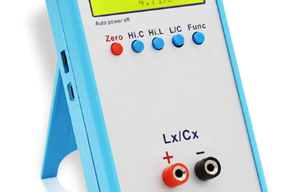
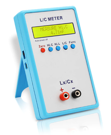
When designing or debugging an electrical or electronics device, it is very important to know the values of the components that have been used on board. With a multimeter most of the components can be easily measured and identified but most ordinary multimeters do not have options to measure inductors and capacitors as this is rarely needed. However, without capacitors there are literally no circuits while complex circuits may have inductors in them. A LCR (inductor-capacitor-resistor) measurement meter can be used to determine the aforementioned components but usually such meters are pretty expensive.
A pyranometer or solar irradiation tester is measurement tool that is a must-have for every professional in renewable energy sector. However, owing one is not easy because it is both expensive and rare. It is expensive because it uses highly calibrated components and it is rare because it is not an ordinary multi-meter that is available in common hardware shops.
Personally, I
have a long professional career in the field of LED lighting, renewable energy
(mainly solar), Lithium and industrial battery systems, electronics and
embedded-systems. I have been at the core of designing, testing, commissioning
and analyzing some of the largest solar power projects of my country – a
privilege that only a few enjoyed. In many of my solar-energy endeavors, I
encountered several occasions that required me to estimate solar isolation or
solar irradiation. Such situations included testing solar PV module
efficiencies, tracking solar system performance with seasons, weather, sky
conditions, dust, Maximum Power Point Tracking (MPPT) algorithms of solar
inverters, chargers, etc.
I wanted a
simply way with which I can measure solar irradiance with some degree of
accuracy. Having the advantage of working with raw solar cells, tools that test
cells and complete PV modules combined with theoretical studies, I found out a
rudimentary method of measuring solar irradiation.
In simple terms, solar insolation is defined as the amount of solar radiation incident on the surface of the earth in a day and is measured in kilowatt-hour per square meter per day (kWh/m²/day). Solar irradiation, on the other hand, is the power per unit area received from the Sun in the form of electromagnetic radiation as measured in the wavelength range of the measuring instrument. It is measured in watt per square meter (W/m²). The solar insolation is, therefore, an aggregate of solar irradiance over a day. Sun energy collection by solar photovoltaic (PV) modules is depended on solar irradiance and this in turn has impact on devices using this energy. For example, in a cloudy day a solar battery charger may not be able to fully charge a battery attached to it. Likewise, in a sunny day the opposite may come true.
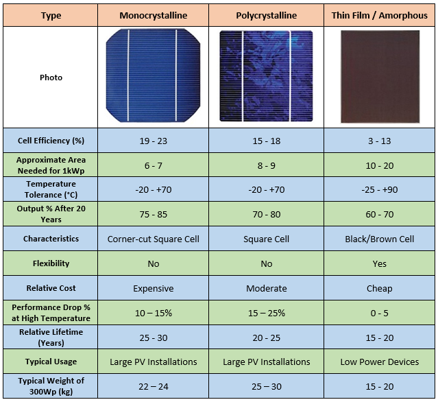
Solar PV Cells
For making a solar irradiation meter we would obviously need a solar cell. In terms of technology, there are three kinds of cells commonly available in the market and these are shown below.
Basic Solar Math
Typically, Earth-bound solar irradiation is about 1350 W/m². About 70 – 80% of this irradiation makes to Earth’s surface and rest is absorbed and reflected. Thus, the average irradiation at surface is about 1000 W/m². Typical cell surface area of a poly crystalline cell having dimensions 156 mm x 156 mm x 1mm is:
The theoretical or ideal wattage of such a cell should be:
However, the present-day
cell power with current technology somewhere between 4 – 4.7 Wp. It is safe to
assume an average wattage of a typical poly crystalline cell to be 4.3 Wp.
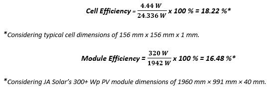
Therefore, cell efficiency is calculated to be:
72 cells of 4.3 Wp capacity will
form a complete solar PV module of 310Wp.
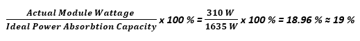
Likewise, the approximate area of a 310 Wp solar panel having dimensions (1960 mm x 991 mm x 40 mm) is:
The theoretical wattage that we should be getting with 1.942 m² area panel is found to be:
Therefore, module/panel efficiency is calculated to be:
Cell efficiency is always higher than module efficiency because in a complete PV module there are many areas where energy is not harvested. These areas include bus-bar links, cell-to-cell gaps, guard spaces, aluminum frame, etc. As technology improves, these efficiencies also improve.
Monocrystalline cells have same
surface are but more wattage, typically between 5.0 to 5.5 Wp. We can assume an
average cell wattage of 5.2 Wp.
Therefore, cell efficiency is calculated to be:
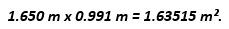
Typically, monocrystalline PV modules consist of 60 cells and so 60 such cells are arranged then the power of a complete PV module is calculated to be:
The area of that PV module having dimensions 1650 mm x 991 mm x 38 mm would be:
The theoretical wattage that we should be getting with 1.635 m² area panel is found to be:
Therefore, module/panel efficiency is calculated to be:
These calculations prove the
following points:
Monocrystalline PV modules can harvest the same amount of energy as their polycrystalline counterparts with lesser area.
Monocrystalline cells are more efficient than poly crystalline cells.
Monocrystalline PV modules are more efficient than polycrystalline PV modules.
156 mm x 156 mm cell dimension is typical but there are also cells of other dimensions like 125 mm x 125 mm x 1 mm.
Though I compared monocrystalline and polycrystalline cells and modules here the same points are true for thin film or amorphous cells.
Currently, there are more efficient cells and advanced technologies, and thus higher power PV modules with relatively smaller area. For instance, at present there are PV modules from Tier 1 manufacturers that have powers well above 600W but their physical dimensions are similar to 300Wp modules.
Solar PV modules can be generally categorized in four categories based on the number of solar cells in series and they usually have the following characteristics:
36 Cells
36
x 0.6 V = 21.6V (i.e., 12V Panel)
VOC
= 21.6V
VMPP
= 16 – 18V
For
modules from 10 – 120 Wp
60 Cells
60
x 0.6 V = 36V
VOC
= 36V
VMPP
= 25 – 29V
For
modules from 50 – 300+ Wp
72 Cells
72
x 0.6 V = 43.2V (i.e., 24V Panel)
VOC
= 43.2V
VMPP
= 34 – 38V
For
modules from 150 – 300+ Wp
96 Cells
96
x 0.6 V = 57.6V (i.e., 24V Panel)
VOC
= 57.6V
VMPP
= 42 – 48V
For
modules from 250 – 300+ Wp
Rare
One cell may not be fully used and could be cut with laser scribing machines to meet voltage and power requirements. Usually, the above-mentioned series connections are chosen because they are the standard ones. Once a cell series arrangement is chosen, the cells are cut accordingly to match required power. A by-cut cell has lesser area and therefore lesser power. Cutting a cell reduces its current and not its voltage. Thus, power is reduced. 36 cell modules are also sometimes referred as 12V panels although there is no 12V rating in them and this is because such modules can directly charge a 12V lead-acid battery but cannot charge 24V battery systems without the aid of battery chargers. Similarly, 72 cell modules are often referred as 24V panels.
Important Parameters of a Panel/Cell
Open Circuit Voltage (Voc) –no load/open-circuit voltage of cell/panel.
Short Circuit Current (Isc) – current that will flow when the panel/cell is shorted in full sunlight.
Maximum Power Point Voltage (VMPP) – output voltage of a panel at maximum power point or at rated power point of the cell’s/panel’s characteristics curve.
Maximum Power Point Current (IMPP) – output current of a panel at maximum power point or at rated power point of the cell’s/panel’s characteristics curve.
Peak Power (Pmax) – the product of VMPP and IMPP. It is the rated power of a cell’s/PV module at STC. Its unit is watt-peak (WP) and not watts because this is the maximum or peak power of a cell/module.
Power Tolerance – percentage deviation of power.
STC stands for Standard Temperature Condition or simply lab conditions (25°C).
AM stands for Air Mass – This can be used to help characterize the solar spectrum after solar radiation has traveled through the atmosphere.
E stands for Standard Irradiation of 1000 W/m².
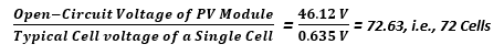
Shown below is the technical specification sticker of a 320 Wp JA Solar PV Module:
According to the sticker the PV module has the following
specs at STC and irradiation, E = 1000 W/m²:
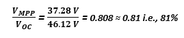
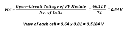
VOC = 46.12 V
VMPP = 37.28 V
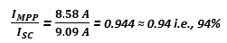
Isc = 9.09 A
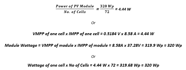
IMPP = 8.58 A
Pmax = 320 WP
From these specs we can estimate and deduce the followings:
VMPP-by-VOC ratio:
This value is always between 76 – 86%.
Similarly, IMPP-by-ISC ratio:
This value is always between 90 – 96%.
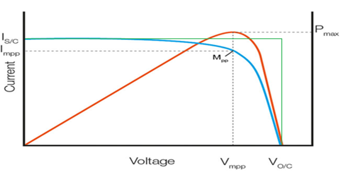
The product of these ratios should be as high as possible. Typical values range between 0.74 – 0.79. This figure represents fill-factor (FF) of a PV module or a PV cell.
An ideal
PV cell/module should have a characteristics curve represented by the green
line. However, the actual line is represented by the blue one. Fill-Factor is
best described as the percentage of ideality. Thus, the greater it is or the
closer it is to 100 % the better is the cell/module.
In this case, the FF is calculated to be 0.94 x 0.81 = 0.76 or 76%.
Number of cells is calculated to be:
Therefore, each cell has an open circuit voltage (VOC) of:
IMPP is 8.58 A and
ISCis 9.09 A.
Cell power is calculated as follows:
Efficiencies are deduced as follows:
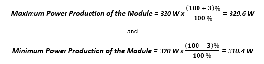
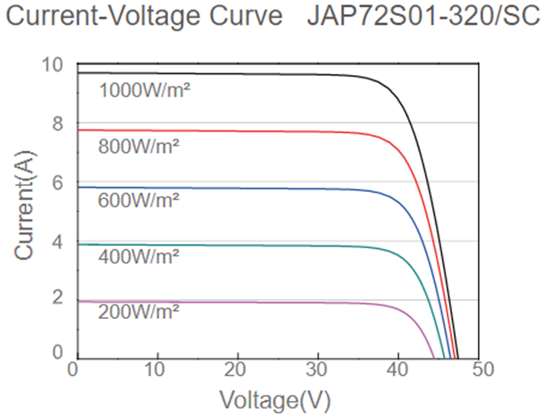
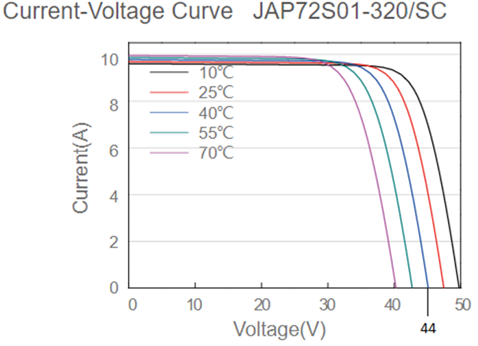
The I-V curves of the PV module shown below show the effect of solar irradiation on performance. It is clear that with variations in solar irradiation power production varies. The same is shown by the power curve. Voltage and current characteristics follow a similar shape.
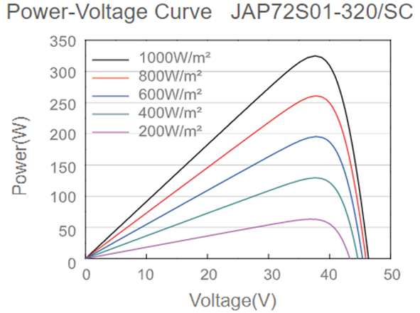
The I-V curve shown below demonstrates the effect of temperature on performance. We can see that power production performance deteriorates with rise in temperature.
The characteristics curves of the
320 Wp JA Solar PV module are shown above. From the curves above we can clearly
see the following points:
Current changes with irradiation but voltage changes slightly and so power generation depends on irradiation and current.
Current changes slightly with temperature but voltage changes significantly. At high temperatures, PV voltage decreases and this leads to change in Maximum Power Point (MPP) point. Thus, at high temperatures power generation decreases and vice-versa.
Vmpp-by-Voc ratio remains pretty much the same at all irradiation levels.
The curves are similar to that of a silicon diode and this is so because a cell is essentially a light sensitive silicon diode.
Impacts of Environment on PV
Effect of Temperature
Let us now see how temperature affects solar module performance. Remember that a solar cell is just like a silicon diode and we know that a silicon diode’s voltage changes with temperature. This change is about -2 mV/°C. Thus, the formula below demonstrates the effect of temperature:
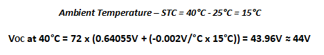
Suppose the ambient temperature is 35°C and let us consider the same 320 Wp PV module having:
VOC at STC = 46.12V
VMPP at STC = 37.28V
Therefore, the temperature difference from STC is:
Under such
circumstance the VMPP
should be about 35V but it gets decreased more and fill-factor is ultimately
affected.
So clearly there is a shift in VMPP which ultimately affects output power. This is also shown in the following graph:
Effect of Shading, Pollution and Dust
Power generation is also affected by shades, i.e., obstruction of
sunlight. Obstacles can be anything from a thin stick to a large tree. Dust and
pollution also contribute to shading on microscopic level. However, broadly
speaking, shading can be categorized in two basic categories – Uniform Shading
and Non-uniform Shading.
Uniform shading is best described as complete shading of all PV modules
or cells of a solar system. This form of shading is mainly caused by dust,
clouds and pollution. In such shading conditions, PV current is affected
proportionately with the amount of shading, yielding to decreased power
collection. However, fill-factor and efficiencies are literally unaffected.
Non-uniform shading, as its name suggests, is partial shading of some PV modules or cells of a solar system. Causes of such shading include buildings, trees, electric poles, etc. Non-uniform shading must be avoided because cells that receive less radiation than the others behave like loads, leading to formation of hotspots in long-run. Shadings as such result in decreased efficiency, current and power generation because of multiple wrong MPP points.
Effect of Other Variables
There are several other variables that have effect on solar energy collection. Variables and weather conditions like rain, humidity, snow, clouds, etc. affect energy harvest while cool, windy and sunny conditions have positive impact on energy harvest. These factors are region and weather dependent and cannot be generalized.
Basic Solar Geometry
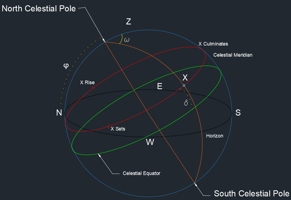
Some basics of solar geometry is needed to be realized to efficiently design solar systems and how sun rays are reach earth. Nature follows a mathematical pattern that it never suddenly or abruptly alters. The movement of the sun and its position on the sky at any instance can be described by some simple trigonometric functions. The Earth not just orbits the Sun but it tilts and revolves about its axis. The daily rotation of the Earth about the axis through its North and South poles (also known as celestial poles) is perpendicular to the equator point, however it is not perpendicular to the plane of the orbit of the Earth. In fact, the measure of tilt or obliquity of the axis of the Earth to a line perpendicular to the plane of its orbit is currently about 23.5°.
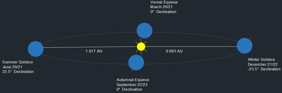
The plane of the Sun is the plane parallel to the Earth’s celestial equator and through the center of the sun. The Earth passes alternately above and below this plane making one complete elliptic cycle every year.
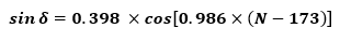
In summer solstice, the Sun shines down most directly on the Tropic of Cancer in the northern hemisphere, making an angle δ = 23.5° with the equatorial plane. Likewise, in winter solstice, it shines on the Tropic of Capricorn, making an angle δ = -23.5° with the equatorial plane. In equinoxes, this angle δ is 0°. Here δ is called the angle of declination. In simple terms the angle of declination represents the amount of Earth’s tilt or obliquity.
The angle of declination, δ, for Nth day of a year can be deduced using the following formula:
Here, N = 1
represents 1st January.
The angle of
declination has effect on day duration, sun travel path and thus it dictates
how we should tilt PV modules with respect to ground with seasonal
changes.
The next most important thing to note is the geographical location in terms of GPS coordinates (longitude, λ East and latitude, ϕ North). This is because geo location also has impact on the aforementioned. Northern and Southern Hemispheres have several differences.
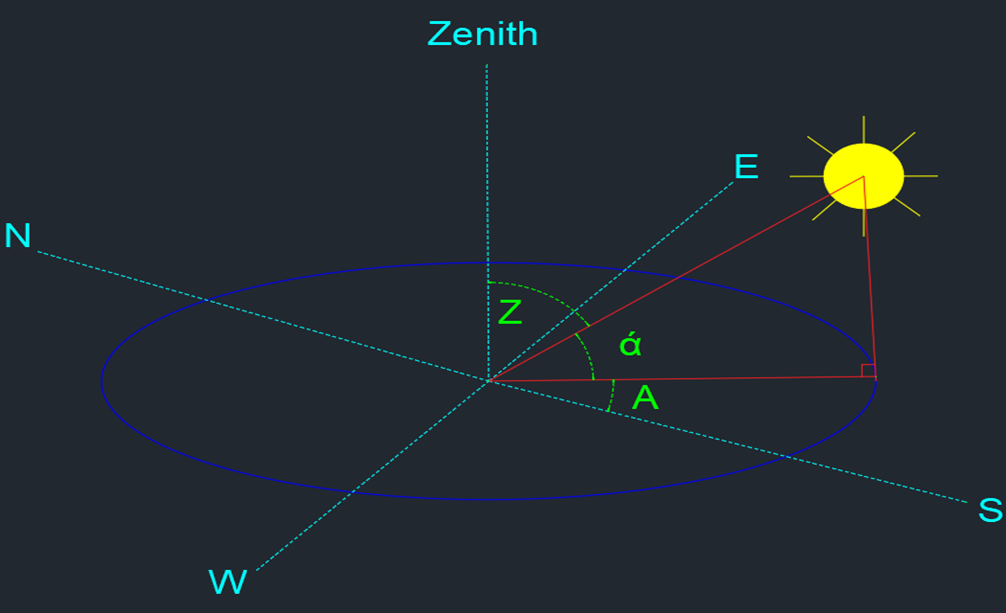
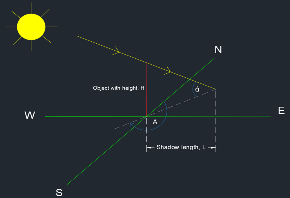
Shown below is
a graphical representation of some other important solar angles. Here:
The angle of solar elevation, ά,
is the angular measure of the Sun’s rays above the horizon.
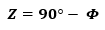
The solar zenith angle, Z, is
the angle between an imaginary point directly above a given location, on the
imaginary celestial
sphere. and the center of the Sun‘s disc. This is
similar to tilt angle.
The azimuth angle, A, is a local
angle between the direction of due North and that of the perpendicular projection
of the Sun down onto the horizon line measured clockwise.
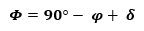
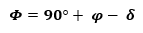
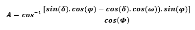
The angle of solar elevation, ά, at noon for location on Northern Hemisphere can be deduced as follows:
Similarly, for location on Southern Hemisphere, the angle of solar elevation at noon can be deduced as follows:
Here ϕ represents latitude and δ represents angle of declination. Zenith/Tilt angle is found to be:
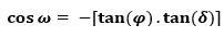
Determining azimuth angle is not simple as additional info are needed. The first thing that we will need is to the sunrise equation. This is used to determine the local time of sunrise and sunset at a given latitude, ϕ at a given solar declination angle, δ. The sunrise equation is given by the formula below:
Here ω is the hour angle. ω is between -180° to 0° at
sunrise and between 0° to 180° at sunset.
If [tan(ϕ).tan(δ)] ≥
1, there is no sunset on that day. Likewise, if [tan(ϕ).tan(δ)] ≤
-1, there is no sunrise on that day.
The hour angle, ω is the
angular distance between the meridian of the observer and the meridian whose
plane contains the sun. When the sun reaches its highest point in the sky at noon, the hour angle is zero. At this time the Sun is said to be ‘due south’ (or ‘due north’, in the Southern Hemisphere) since the meridian plane of the observer contains the Sun. On every hour the hour angle increases by 15°.
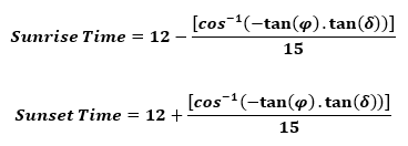
From hour angle, we can determine the local sunrise and sunset times as follows:
For a given location, hour angle and date the angle of solar elevation can be expressed as follows:
Since we have the hour angle info along with sunrise and sunset times, we can now determine the azimuth angle. It is expressed as follows:
Solving the above equation for A will yield in azimuth angle.
Knowing azimuth and solar elevation angles help us determine the length and location of the shadow of an object. These are important for solar installations.
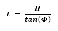
The length of the shadow is as in the figure above is found to be:
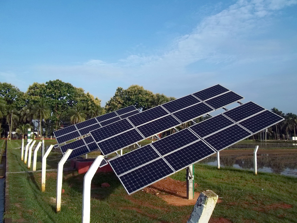
From the geometric analysis, it can be shown that solar energy harvest will increase if PV modules can be arranged as such to follow the Sun. This is the concept of solar tracking system.
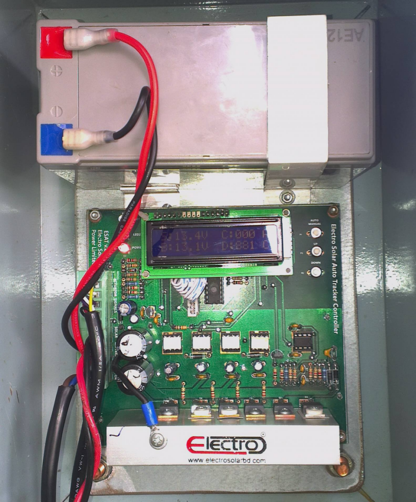
If the Sun can be tracked according to these math models, the maximum possible harvest can be obtained. However, some form of solar-tracking structures will be needed. An example of sun tracking system is shown above. This was designed by a friend of mine and myself back in 2012. He designed the mechanical section while I added the intelligence in form of embedded-system coding and tracking controller design.
Here’s a photo of the sun tracking controller that I designed. It used a sophisticate algorithm to track the sun.
Building the Device
In order to
build the solar irradiance meter, we will need a solar cell or a PV module of
known characteristics. Between a single cell and module, I would recommend for
a cell because:
Cells have lower power than complete modules.
Cells have almost no framing structure.
Cells are small and light-weight.
Cells are individual and so there is no need to
take account of series-parallel combination.
We would see
why these are important as we move forward.
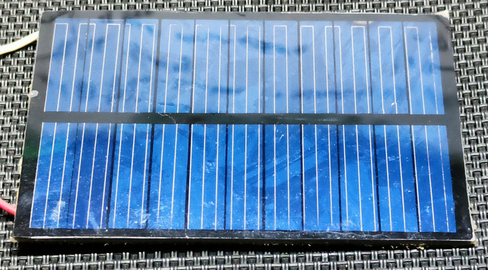
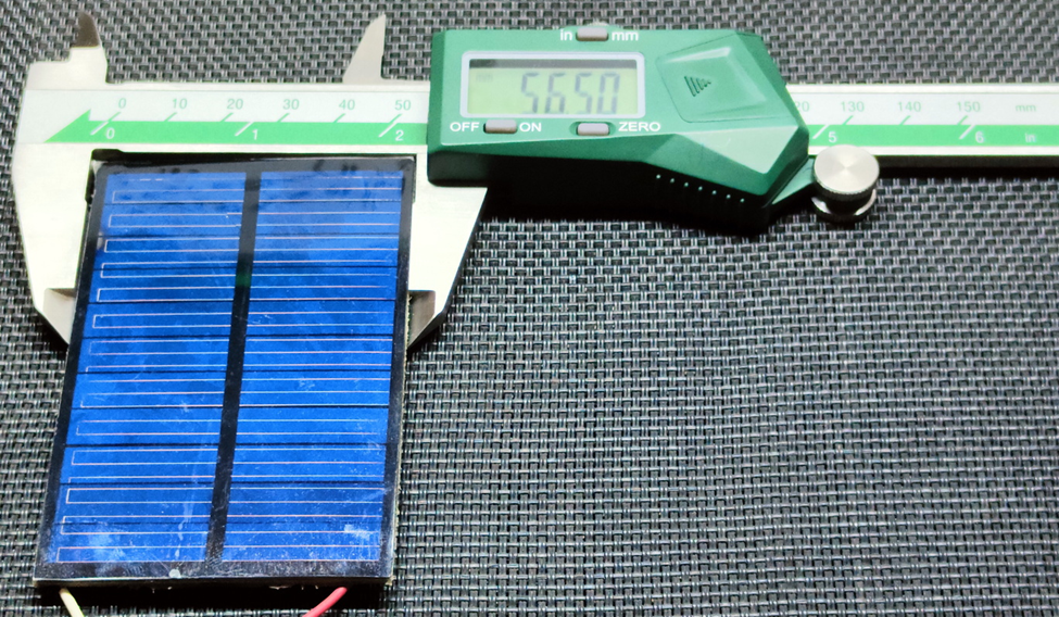
For the project, I used a cheap amorphous solar cell as shown in the photo below. It looks like a crystalline cell under my table lamp but actually it is an amorphous one. It can be purchased from AliExpress, Amazon or similar online platform.
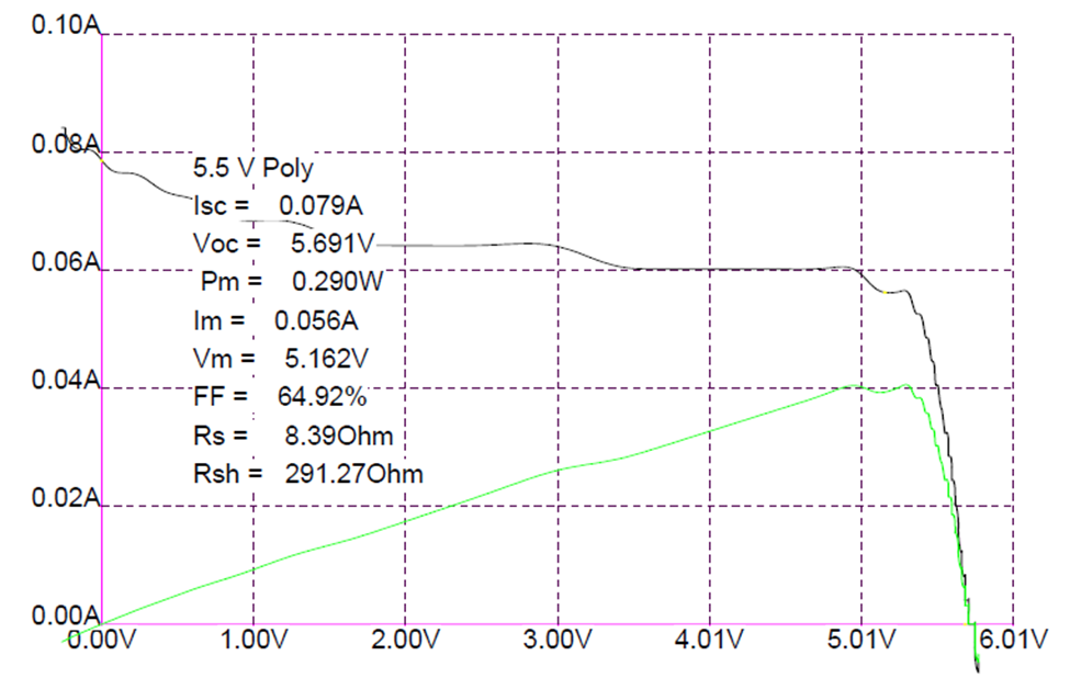
With a cell test machine, it gave a characteristic curve and data as shown below:
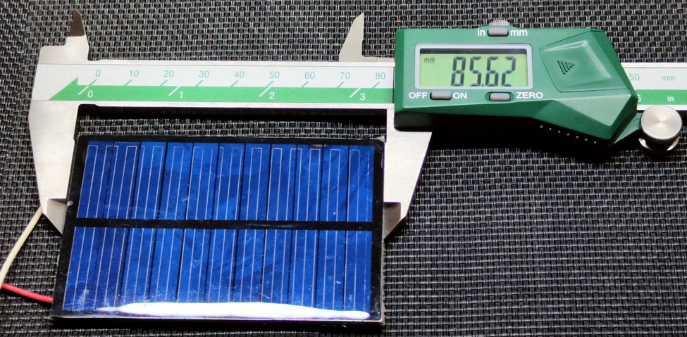
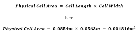
From this I-V characteristics curve, we can see its electrical parameters. The cell has a physical dimension of 86mm x 56mm and so it has an area of 0.004816m².
From the calculation which I
already discussed, irradiation measurement needs two known components – the
total cell area and the maximum power it can generate. We know both of these
data. Now we just have to formulate how we can use these data to measure
irradiation.
Going back to a
theory taught in the first year of electrical engineering, the
maximum power transfer theorem, we know that to
obtain maximum external power from a source with a finite internal resistance, the resistance of the load
must equal the resistance of the source as viewed from its output terminals.
This is the theory behind my irradiation measurement.
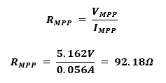
From the cell
electrical characteristics data, we can find the ideal resistance that is
needed to make this theory work.
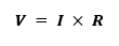
It is important to note that we would just be focusing on maximum power point data only and that is because this is the maximum possible output that the cell will provide at the maximum irradiation level of 1000W/m². The ideal resistance is calculated as follows:
and so does the electric current. The voltage that would be induced across RMPP is proportional to this current because according to Ohms law:
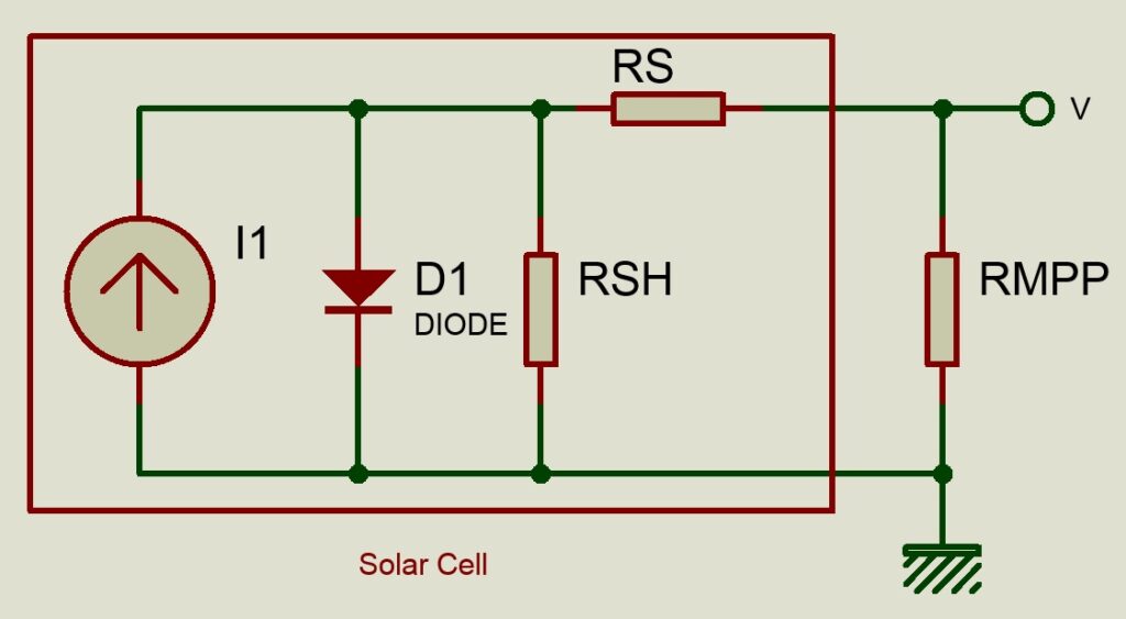
The equivalent circuit is as shown below:
The boxed
region is the electrical equivalent of a solar cell. At this point it may look
complicated but we are not digging inside the box and so it can be considered
as a mystery black box.
We know that:
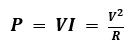
We know the value of resistance and all we have to do is to measure the voltage (V) across the cell. We also know the area of the cell and so we can deduce the value of irradiation, E incident on the cell according to the formula:
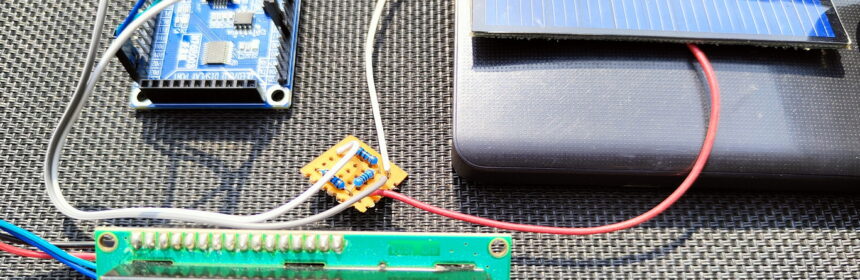
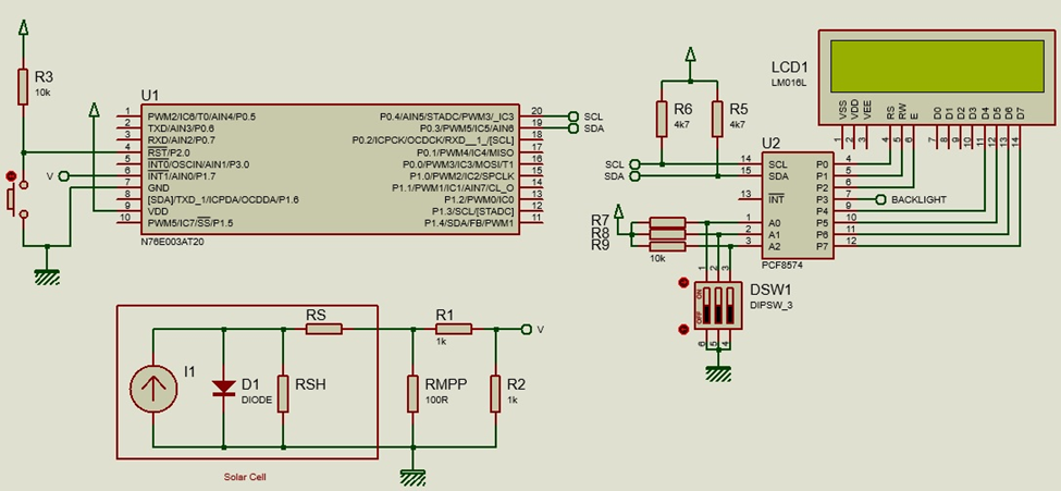
This project is
completed with a Nuvoton N76E003 microcontroller. I chose this microcontroller because
it is cheap and features a 12-bit ADC. The high-resolution ADC is the main reason
for using it because we are dealing with low power and thus low voltage and
current. The solar cell that I used is only about 300mW in terms of power. If
the reader is new to Nuvoton N76E003 microcontroller, I strongly suggest going
through my tutorials on this microcontroller here.
Let us first see what definitions have been used in the code. Most are self-explanatory.
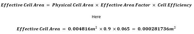
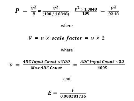
#define cell_efficiency 0.065F // 6.5% (Typical Amorphous Cell Efficiency) #define cell_length 0.0854F // 85.4mm as per inscription on the cell #define cell_width 0.0563F // 56.3mm as per inscription on the cell #define effective_area_factor 0.90F // Ignoring areas without cell, i.e. boundaries, frames, links, etc #define cell_area (cell_length * cell_width) // 0.004816 sq.m #define effective_cell_area (cell_area * effective_area_factor * cell_efficiency) // 0.000281736 sq.m
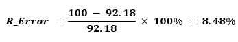
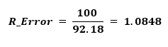
Obviously VMPP and IMPP are needed to calculate RMPP and this is called here as R_actual. R_fixed is the load resistor that is put in parallel to the solar cell and this is the load resistor needed to fulfill maximum power transfer theorem. Practically, it is not possible to get 92.18Ω easily and so instead of 92.18Ω ,a 100Ω (1% tolerance) resistor is placed in its place. The values are close enough and the difference between these values is about 8%. This difference is also taken into account in the calculations via the definition R_Error.
Thus, during calculation this amount of difference should be compensated for.
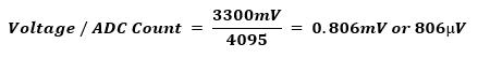
ADC_Max and VDD are maximum ADC count and supply voltage values respectively. These would be needed to find the voltage resolution that the ADC can measure.
Since 806µV
is a pretty small figure, we can rest assure that very minute changes in solar
irradiance will be taken into account during measurement.
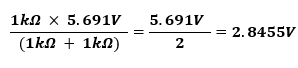
scale_factor is the voltage divider ratio. The cell gives a maximum voltage output of 5.691V but N76E003 can measure up to 3.3V. Thus, a voltage divider is needed.
This
is the maximum voltage that N76E003 will see when the cell reaches open-circuit
voltage. Thus, the ADC input voltage needs to be scaled by a factor of 2 in
order to back-calculate the cell voltage, hence the name scale_factor.
The next definitions are related to the cell that is used in this project. Cell length and width are defined and with these the area of the cell is calculated.
The physical
cell area does not represent the total area that is sensitive to solar irradiation.
There are spaces within this physical area that contain electrical links, bezels
or frame, etc. Thus, a good estimate of effective solar sensitive cell area is
about 90% of the physical cell area. This is defined as the effective_area_factor.
Lastly, we have to take account of cell efficiency because we have seen that in a given area not all solar irradiation is absorbed and so the cell_efficiency is also defined. Typically, a thin film cell like the one I used in this project has an efficiency of 6 – 7% and so a good guess is 6.5%. All of the above parameters lead to effective cell area and it is calculated as follows:
So now the aforementioned equation becomes as follows:
The equations
suggest that only by reading ADC input voltage we can compute both the power
and solar irradiance.
The code initializes by initializing the I2C LCD, printing some fixed messages and enabling ADC pin 0.
The core components of the code are the functions related to ADC reading and averaging. The code below is responsible for ADC reading.
unsigned int ADC_read(void)
{
  register unsigned int value = 0x0000;

  clr_ADCF;
  set_ADCS;
  while(ADCF == 0);

  value = ADCRH;
  value <<= 4;
  value |= ADCRL;

  return value;
}
The following code does the ADC averaging part. Sixteen samples of ADC reading are taken and averaged. Signal averaging allows for the elimination of false and noisy data. The larger the number of samples, the more is the accuracy but having a larger sample collection lead to slower performance.
unsigned int ADC_average(void)
{
    signed char samples = 16;
    unsigned long value = 0;

    while(samples > 0)
    {
        value += ((unsigned long)ADC_read());
        samples--;
    };

    value >>= 4;

    return ((unsigned int)value);
}
In the main, the ADC average is read and this is converted to voltage. The converted voltage is then upscaled by applying the scale_factor to get the actual cell voltage. With the actual voltage, power and irradiation are computed basing on the math aforementioned. The power and irradiation values are displayed on the I2C LCD and the process is repeated every 100ms.
ADC = ADC_average(); v = ((VDD * ADC) / ADC_Max); V = (v * scale_factor); P = (((V * V) / R_fixed) * R_Error); E = (P / effective_cell_area);
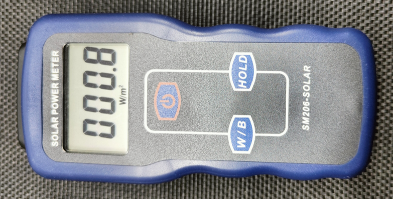
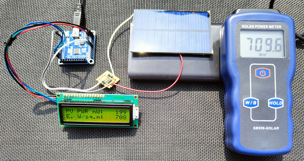
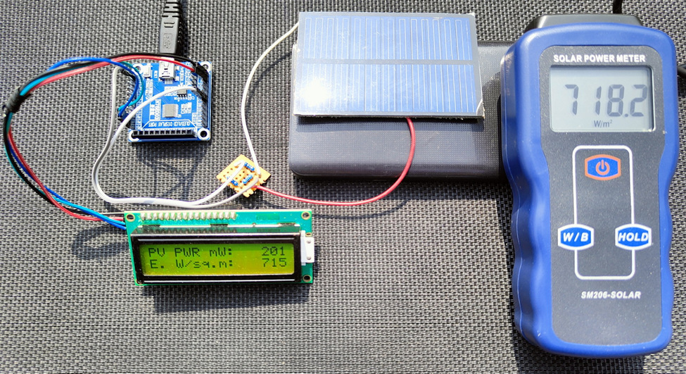
I have tested the device against a SM206-Solar solar irradiation meter and the results are fairly accurate enough for simple measurements.
Demo
Demo video links:
Improvements and Suggestions
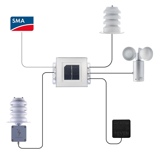
Though this device is not a professional solar irradiation measurement meter, it is fair enough for simple estimations. In fact, SMA – a German manufacturer of solar inverter, solar charger and other smart solar solution uses a similar method with their SMA Sunny Weather Station. This integration allows them to monitor their power generation devices such as on-grid inverters, multi-cluster systems, etc. and optimize performances.
There are rooms for lot of improvements
and these are as follows:
A temperature sensor can be mounted on the backside of the solar cell. This sensor can take account of temperature variations and thereby compensate readings. We have seen that temperature affects solar cell performance and so temperature is a major influencing factor.
A smaller cell would have performed better but it would have needed additional amplifiers and higher resolution ADCs. A smaller cell will have lesser useless areas and weight. This would make the device more portable.
Using filters to filter out unnecessary components of solar spectrum.
Adding a tracking system to scan and align with the sun would result in determining maximum irradiation.
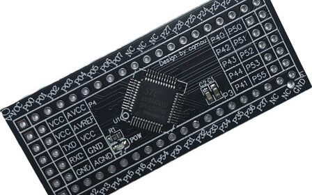
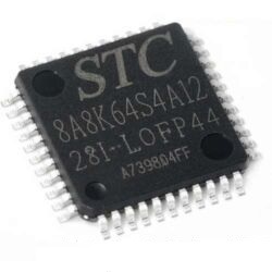
About STC8A8K64S4A12
Microcontroller and its Development Board
This is the continuation of my first post on STC 8051 Microcontrollers here.
Many Chinese microcontroller manufacturers develop awesome and cheap general-purpose MCUs using the popular 8051 architecture. There are many reasons for that but most importantly the 8051 architecture is a very common one that has been around for quite a long time. Secondly, manufacturing MCUs with 8051 DNA allows manufacturers to focus less on developing their own proprietary core and to give more effort in adding features. Holtek, Nuvoton, STC, etc are a few manufacturers to name.
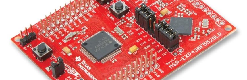
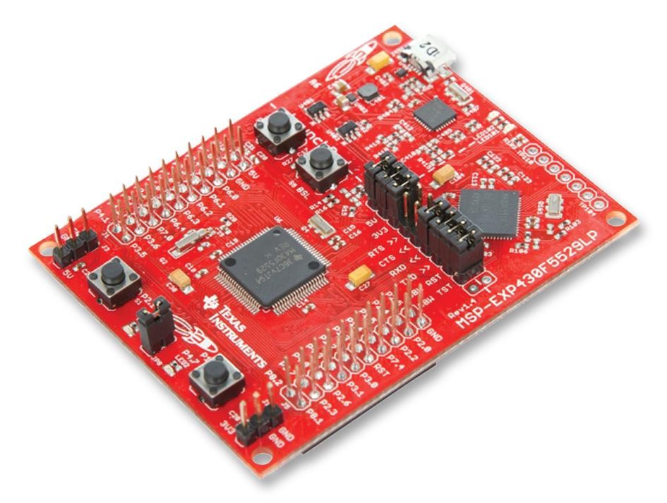
In my past tutorials on MSP430s, I demonstrated how to get started with MSP430 general purpose microcontrollers from Texas Instruments (TI). Those tutorials covered most aspects of low and mid-end MSP430G2xxx series microcontrollers. For those tutorials, TI’s official software suite – Code Composer Studio (CCS) – an Eclipse-based IDE and GRACE – a graphical peripheral initialization and configuration tool similar to STM32CubeMX were used. To me, those low and mid-end TIs chips are cool and offer best resources one can expect at affordable prices and small physical form-factors. I also briefly discussed about advanced MSP430 microcontrollers and the software resources needed to use them effectively. Given these factors, now it is high time that we start exploring an advanced 16-bit TI MSP430 microcontroller using a combination of past experiences and advanced tools. MSP430F5529 is such a robust high-end device and luckily it also comes with an affordable Launchpad board dedicated for it.